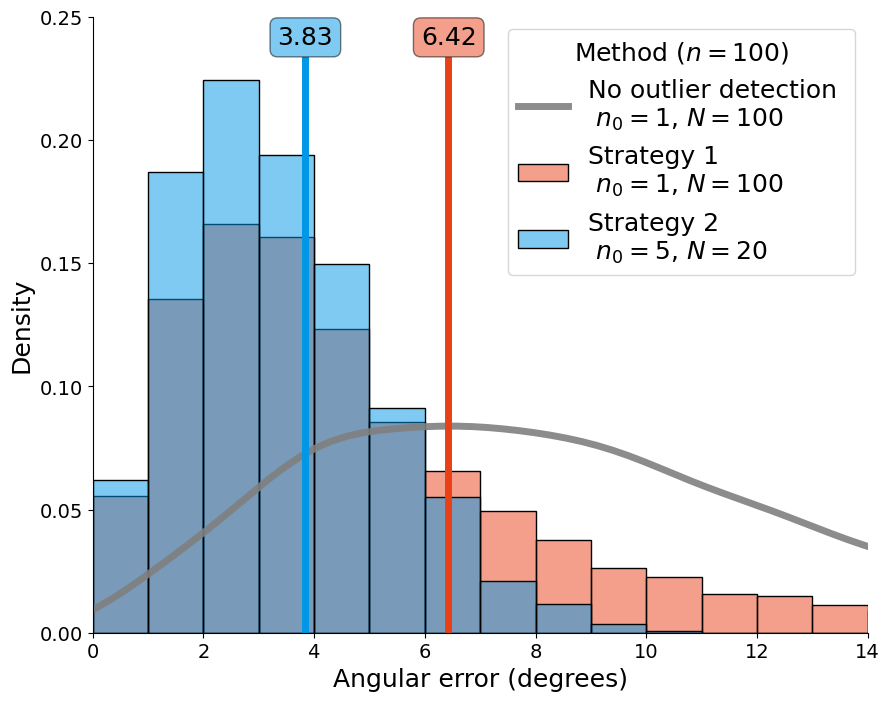
Figure 3: Histogram comparing sampling strategies

import numpy as np
import pandas as pd
import matplotlib.pyplot as plt
import seaborn as sns

import pmagpy.pmag as pmag
import pmagpy.ipmag as ipmag

import smpsite as smp

import warnings 
warnings.filterwarnings('ignore')

%matplotlib inline

Run simulation

This notebook also includes how to run the simulation for the histograms.

%%time

angular_dispersio_within_site = 10 # degrees
kappa_within_site = smp.angular2kappa(angular_dispersio_within_site)
latitude = 30
outlier_rate = 0.10
n_iters = 5000

params1 = smp.Params(N=100,
                     n0=1,
                     kappa_within_site=kappa_within_site,
                     site_lat=latitude, 
                     site_long=0,
                     outlier_rate=outlier_rate,
                     secular_method="G",
                     kappa_secular=None)

params2 = smp.Params(N=20,
                     n0=5,
                     kappa_within_site=kappa_within_site,
                     site_lat=latitude, 
                     site_long=0,
                     outlier_rate=outlier_rate,
                     secular_method="G",
                     kappa_secular=None)

df_false    = smp.simulate_estimations(params1, n_iters=n_iters, ignore_outliers="False")
df_true     = smp.simulate_estimations(params2, n_iters=n_iters, ignore_outliers="True")
df_vandamme = smp.simulate_estimations(params1, n_iters=n_iters, ignore_outliers="vandamme")

df_false.to_csv("../../outputs/fig3a_df_false.csv")
df_true.to_csv("../../outputs/fig3a_df_true.csv") 
df_vandamme.to_csv("../../outputs/fig3a_df_vandamme.csv") 

CPU times: user 33min 41s, sys: 123 ms, total: 33min 41s
Wall time: 33min 41s

Figure

# panel = 'a'
# panel = 'b'
panel = 'c'

df_false = pd.read_csv("../../outputs/fig3"+panel+"_df_false.csv")
df_true = pd.read_csv("../../outputs/fig3"+panel+"_df_true.csv")
df_vandamme = pd.read_csv("../../outputs/fig3"+panel+"_df_vandamme.csv")

df_true

	Unnamed: 0	plong	plat	total_samples	samples_per_sites	S2_vgp	error_angle	S2_vgp_real	n_tot	N	n0	kappa_within_site	site_lat	site_long	outlier_rate	secular_method	kappa_secular	ignore_outliers
0	0	190.306018	84.314629	36.0	5	218.096967	5.685371	191.7229	100	20	5	66.069981	30	0	0.6	G	NaN	True
1	1	55.662167	85.483652	34.0	5	215.659161	4.516348	191.7229	100	20	5	66.069981	30	0	0.6	G	NaN	True
2	2	193.984859	86.462183	34.0	5	265.162109	3.537817	191.7229	100	20	5	66.069981	30	0	0.6	G	NaN	True
3	3	358.720274	86.835100	34.0	5	461.786418	3.164900	191.7229	100	20	5	66.069981	30	0	0.6	G	NaN	True
4	4	224.066484	87.495521	28.0	5	206.023724	2.504479	191.7229	100	20	5	66.069981	30	0	0.6	G	NaN	True
...	...	...	...	...	...	...	...	...	...	...	...	...	...	...	...	...	...	...
4995	4995	165.292979	84.319601	39.0	5	121.964481	5.680399	191.7229	100	20	5	66.069981	30	0	0.6	G	NaN	True
4996	4996	9.619776	87.047602	46.0	5	175.154300	2.952398	191.7229	100	20	5	66.069981	30	0	0.6	G	NaN	True
4997	4997	338.354021	85.822482	40.0	5	163.134369	4.177518	191.7229	100	20	5	66.069981	30	0	0.6	G	NaN	True
4998	4998	14.220743	87.025506	48.0	5	163.107882	2.974494	191.7229	100	20	5	66.069981	30	0	0.6	G	NaN	True
4999	4999	137.642242	86.984741	41.0	5	301.022274	3.015259	191.7229	100	20	5	66.069981	30	0	0.6	G	NaN	True

5000 rows × 18 columns

%matplotlib inline

if panel == 'a':
    x_max = 8
    y_max = 0.52
    bw = 0.5
elif panel == 'b':
    x_max = 8
    y_max = 0.4
    bw = 0.5
elif panel == 'c':
    x_max = 14
    y_max = 0.25
    bw = 1.0

fig, axes = plt.subplots(nrows=1, ncols=1, figsize=(10,8))

# Histograms
sns.histplot(df_vandamme.error_angle, ax=axes, color='#e84118', stat='density', binwidth=bw, binrange=(0,20), alpha=.5, label="Strategy 1 \n $n_0=1$, $N=100$")
sns.histplot(df_true.error_angle, ax=axes, color='#0097e6', stat='density', binwidth=bw, binrange=(0,20), alpha=.5, label="Strategy 2 \n $n_0=5$, $N=20$")

# Density plot
sns.kdeplot(df_false.error_angle, ax=axes, color='grey', alpha=.9, lw=5, label="No outlier detection \n $n_0=1$, $N=100$")


rmse1 = np.round(np.mean(df_vandamme.error_angle**2)**.5, decimals=2)
rmse2 = np.round(np.mean(df_true.error_angle**2)**.5, decimals=2)

plt.axvline(x=rmse1, ymax=0.93, c='#e84118', lw=5)
plt.axvline(x=rmse2, ymax=0.93, c='#0097e6', lw=5)

props = dict(boxstyle='round', facecolor="#e84118", alpha=0.5)
plt.text(rmse1/x_max-0.035, 0.986, "{}".format(rmse1), transform=axes.transAxes, fontsize=18,
        verticalalignment='top', bbox=props);

props = dict(boxstyle='round', facecolor='#0097e6', alpha=0.5)
plt.text(rmse2/x_max-0.035, 0.986, "{}".format(rmse2), transform=axes.transAxes, fontsize=18,
        verticalalignment='top', bbox=props);

plt.xlim(0, x_max)
plt.ylim(0, y_max)
plt.xlabel("Angular error (degrees)", fontsize=18)
plt.ylabel("Density", fontsize=18)
plt.xticks(np.arange(0.0, x_max+0.1, 2.0), fontsize=14);
plt.yticks(fontsize=14)
plt.legend(title="Method ($n=100$)", title_fontsize=18, fontsize=18)

ax = plt.gca()
ax.spines[['right', 'top']].set_visible(False)

plt.savefig("Figure3{}.pdf".format(panel), format="pdf", bbox_inches='tight')
plt.savefig("Figure3{}.png".format(panel), format="png", bbox_inches='tight')