DIY Figure 1#
In this Do It Yourself (DIY) Figure 1 notebook, one can use the theoretical approximation developed in Sapienza et al. 2023 to change the parameter choices from those illustrated in Figure 1 of the paper associated with pole position estimation. This notebook thereby enables a researcher to obtain estimates of the angular error for the paleopole estimation for the latitude and the estimated within site precision that fits their study.
 |
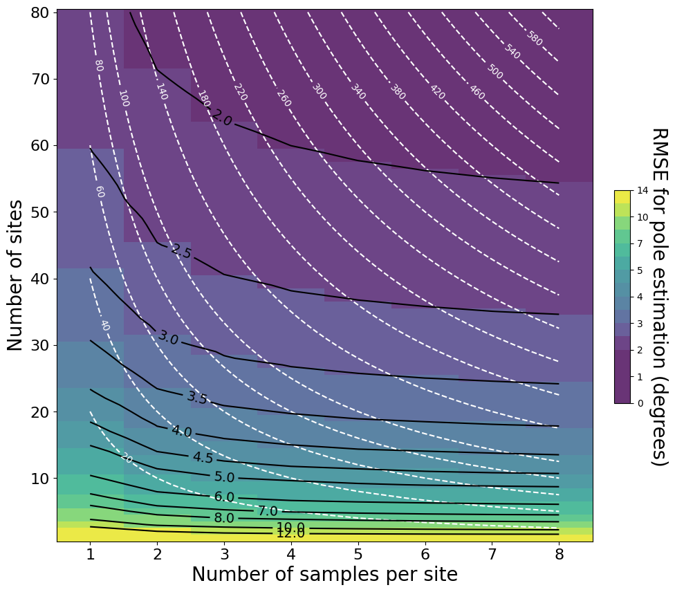
Figure 1: Root mean square error (RMSE) in degrees between site mean poles and the true GAD pole (top panel) and between-site VGP dispersion (bottom panel) as a function of different combinations of the total number of sites N and the number of samples per site n0. For this diagram, we use a paleolatitude of 30° (κb ≈ 35), poutlier = 0, and κw = 50. The white dashed lines represent isolines where the total number of samples n is constant, and the black lines represent isolines with constant net mean error angle. Each point-wise estimate of the mean error (i.e., each box) is based on the results of 10,000 simulations. While these simulations represent secular variation using model G, similar results emerge from using the TK03 model (Tauxe & Kent, 2004). This notebook allows you to recreate the top panel using the theoretical approximation |
A full simulation would be more computationally expensive to run (i.e. take a long time), but our simulations showed that theoretical approximations and numerical simulations differ at most \(1\%\) from each other when there are no outliers in the sample. Therefore, the theoretical approximation is used here.
Import Python packages#
Run this cell to get the Python tools needed for the notebook.
import numpy as np
import pandas as pd
import matplotlib.pyplot as plt
from scipy.ndimage.filters import gaussian_filter
import matplotlib.colors as colors
from itertools import product

import smpsite as smp

%matplotlib inline
/tmp/ipykernel_2380/2317696597.py:4: DeprecationWarning: Please import `gaussian_filter` from the `scipy.ndimage` namespace; the `scipy.ndimage.filters` namespace is deprecated and will be removed in SciPy 2.0.0.
  from scipy.ndimage.filters import gaussian_filter
The parameters of the study location#
The first step is to provide the latitude (site_lat) and longitude (site_long) of the study location (the latitude is what matters).
You also need to provide an estimate of \(\kappa\) which is the Fisher precision parameter for the sample directions within the individual sites of your study. If the directional estimates within a given site are expected to be tightly grouped, this kappa_within_site value will be higher. If they are expected to be more scattered it will be lower.
Change the values below to match the study for which you are interested in exploring sampling strategies
site_lat = 30             # Site latitude
site_long = 0             # Site longitude
kappa_within_site = 50    # Concentration parameter kappa in each site
The number of sites and samples per site to be evaluated#
The maximum number of sites (N_max) and the maximum number of samples per site (n0_max) can be set. In Figure 1 of the paper, N_max`` was 40 and n0_max`` was 20. At values of very high site numbers and/or sample numbers there can be an issue with the code that will result in an error (so keep the values less than a few hundred).
Change the values below to be the number of sites (from 1 to N_max) and number of samples per site (1 to n0_max) that you want to explore in the analysis
N_max = 80 # Maximum values of sites (can go up to ~300)
n0_max = 8  # Maximum values of samples per site
Run the analysis#
The code below will conduct the analysis giving an estimate of the angular mean angular error between estimated poles for a given number of sites and within site samples.
# Create a template data frames with all the combinations of number of sites and samples per site
N_flat = np.tile(np.arange(1, N_max+1, 1), (n0_max,1)).ravel()
n0_flat = np.tile(np.arange(1, n0_max+1, 1), (N_max,1)).T.ravel()

df = pd.DataFrame({'N' : N_flat, 'n0' : n0_flat})

# Compute theoretical error in paleopole estimation

df["error_kappa_theoretical"] = df.apply(lambda row: smp.kappa_theoretical(smp.Params(N=row.N,
                                                                                      n0=row.n0,
                                                                                      kappa_within_site=kappa_within_site,
                                                                                      site_lat=site_lat,
                                                                                      site_long=site_long,
                                                                                      outlier_rate=0.0,
                                                                                      secular_method='G',
                                                                                      kappa_secular=None)), axis=1)

df["error_angle_theoretical"] = df.apply(lambda row: float(smp.kappa2angular(row.error_kappa_theoretical)), axis=1)
df.tail(5)
| N | n0 | error_kappa_theoretical | error_angle_theoretical | |
|---|---|---|---|---|
| 635 | 76 | 8 | 2297.266890 | 1.694923 |
| 636 | 77 | 8 | 2327.494086 | 1.680234 |
| 637 | 78 | 8 | 2357.721282 | 1.665545 |
| 638 | 79 | 8 | 2387.948478 | 1.652216 |
| 639 | 80 | 8 | 2418.175674 | 1.644090 |
Plot the error angle estimates#
The cell below defines a function that will plot the pole angle estimates and then makes that plot. Run the cell below to visualize the results for your chosen parameters.
def find_nearest(A, a0):
    """
    Function to round all the values in a generic numpy array A to the closest value in another array n0.
    """
    a = A.flatten()
    idx = ((np.tile(a, (len(a0),1)).T - a0)**2).argmin(axis=1)
    return a0[idx].reshape(A.shape)

def plot_angle_error(df):

    fig, axes = plt.subplots()
    fig.set_size_inches(10, 10)

    caxes = axes.inset_axes([1.04, 0.26, 0.03, 0.4])

    def contour_plot(df_, ax, cax, bounds, cmap, cbar_title, make_levels=True, make_contours=True,
                     color_max=16, ticks=None, xmax=40):

        X = df_.columns.values
        Y = df_.index.values
        Z = df_.values
        Z_smooth = gaussian_filter(Z, 1.0)

        Z = np.clip(Z, a_min=0.0, a_max=color_max)
        # Z_rounded = np.rint(Z)
        mid_points = (bounds[1:] + bounds[:-1]) / 2
        Z_rounded = find_nearest(Z, mid_points)
        Z_rounded[np.isnan(Z)] = 0

        x,y = np.meshgrid(X, Y)

        if make_levels:
            N = x * y
            levels = np.hstack([np.arange(0.0, 100.0, 20), np.arange(100.0, 1010, 40.)])
            IsoNLines = ax.contour(x, y, N, 10, colors='white', linestyles="dashed", levels=levels)
            ax.clabel(IsoNLines, inline=True, fontsize=10)

        ColorGrid = ax.pcolormesh(x, y, Z_rounded, cmap=cmap, norm=colors.LogNorm(vmin=2, vmax=color_max), alpha=0.8)

        if make_contours:
            ContourLines = ax.contour(x, y, Z, 10, colors='k', levels=bounds)
            ax.clabel(ContourLines, inline=True, fontsize=14)

        # ax.set_xlim([1, n0_max])
        # ax.set_ylim([0, N_max])
        ax.set_xlabel(None)
        ax.set_ylabel(None)
        # ax.set_xticks([1,2,3,4,5,6,7,10,15])
        ax.xaxis.set_tick_params(labelsize=16)
        ax.yaxis.set_tick_params(labelsize=16)

        cbar = plt.colorbar(ColorGrid, cax=cax, boundaries=bounds, orientation='vertical')#, fraction=0.02, location='right')
        cbar.set_label(cbar_title, rotation=270, fontsize=20, labelpad=20)

        return None

    contour_plot(df,
                 axes,
                 cax=caxes,
                 bounds=np.hstack([np.arange(0.0, 5.0, 0.5), np.arange(5.0, 8, 1.0), np.arange(8.0, 16.0, 2.0)]),
                 cmap='viridis',
                 cbar_title="RMSE for pole estimation (degrees)",
                 color_max=14,
                 ticks=[1, 4, 7, 10, 15, 20, 30, 40])

    plt.gca().set_xlabel("Number of samples per site", fontsize=20)
    plt.gca().set_ylabel("Number of sites", fontsize=20)

df_pivot = df.pivot(index='N', columns='n0', values='error_angle_theoretical')

plot_angle_error(df_pivot)